8. Games: Adversarial Search

Until now, we considered the problems that are Single Agent, Fully Observable, Deterministic and Goal-oriented. There are many other problems involving multiple agents, sometimes adversarial to one another. Let us discuss the problems with multiple agents which are adversarial to each other.

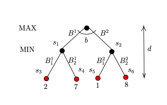
Let us consider the scenario of a two player game. In this game, there are $2$ bags and there are $2$ balls in each bag with a number on it. There are 2 players, one aiming to maximize the score, let us call him/her as MAX player, and the other one is aiming to minimize the score, again let us call him/her as MIN player. The MAX player has to chose a bag, while the MIN player has to choose one ball out of the $2$ balls in the chosen bag. The score is determined by the number on the ball chosen.

Let the 2 bags be $B^1$ and $B^2$ and the 2 balls in bag $B^1$ be $B_1^1$ and $B_1^2$, and the 2 balls in bag $B^2$ be $B_2^1$ and $B_2^2$. The Figure 1 shows the possible outcomes of the game. The red terminal in the Figure 1 represents the balls, and the number on them.

Figure 1: Example of Max-Min 2 player game.

As per Figure 1, $s_0$, the root is the start state of this game, and $s_3, s_4, s_5, s_6$ as indicated by the red nodes are the terminal states where the score of the game is calculated. In addition, we have the 2 parameters depth $d$ and branching factor $b$.

Let utility function be $Utility(s)$ where s is a terminal state, i.e., for example, $Utility(s_3)=2$. The purpose of MAX player is to maximise the utility, while the purpose of MIN player is to minimize the utility.

An intuitive strategy that both players can adopt is to assume that the opponent would play optimally. That is, MAX player would always choose state with the maximum utility, and the MIN player would always choose the minimum utility. Let our transition model function be $RESULT(s,a)$. $RESULT(s,a)$ considers a state $s$ and an action $a$ taken as input to return the next state.

We can derive an algorithm, $MINIMAX(s)$ as follows:

We will now trace this $MINIMAX$ algorithm on the tree in Figure 2 and 3. This will give us the tree below, where nodes are circled when they are explored.

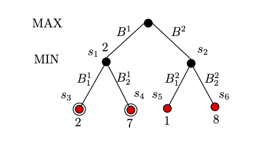
Figure 2: Example to Max-Min 2 player game; Nodes $s_3$ and $s_4$ explored.

• Max player will first explore the $s_3$, and $Utility(s_3) =2$, so at this point, we know that $Utility(s_1) \leq 2$.

• As, Max player does not know the $Utility(s_1)$, it will explore $s_4$, as $Utility(s_4) = 7$, as $Utility(s_1)$ will be decided by Min player, Max player know that the $Utility(s_1)=2$. Refer to Figure 2.

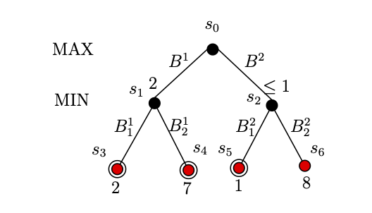
• As shown in Figure 3, the next Max player will check for $s_5$. $Utility(s_5) =1$, so at this point, we know that $Utility(s_2) \leq 1$. From the prospective of Max player, terminal $s_6$ does not exists, as whatever be the Utility of $s_6$, Max player knows that the $Utility(s_2) \leq 1$, as $Utility(s_1)=2$, he should choose $s_1$ over $s_2$.

Figure 3: Example of Max-Min 2 player game; Nodes $s_3$, $s_4$, $s_5$ explored.

Hence, Max player should chose $B_1$ in order to win the game.

8.1. Minimax Algorithm

As discussed in two agent problem, the game can easily be solved by a recursive computation of the minimax values each node in the decision tree, working from the leaves to the root as the recursion unwinds. The algorithm is as follows assuming the MAX player starts first.

Algorithm 1 MinimaxDecision($S$)

1. $bestAction \leftarrow null$
2. $max \leftarrow -\infty$
3. for all action $a$ in ACTIONS($S$) do
4. $~~~~~$ $util \leftarrow$ MinValue(RESULT($S$,$a$))
5. $~~~~~$ if $util > max$ then
6. $~~~~~~~~~~$ $bestAction \leftarrow a$
7. $~~~~~~~~~~$ $max \leftarrow util$
8. return $bestAction$

Algorithm 2 MinValue($S$)

1. if TERMINAL($S$)=True then return UTILITY($S$)
2. $v \leftarrow \infty$
3. for all action $a$ in ACTIONS($S$) do
4. $~~~~~$ $v \leftarrow$ min($v$, MaxValue(RESULT($S$,$a$)))
5. return $v$

Algorithm 3 MaxValue($S$)

1. if TERMINAL($S$)=True then return UTILITY($S$)
2. $v \leftarrow -\infty$
3. for all action $a$ in ACTIONS($S$) do
4. $~~~~~$ $v \leftarrow$ max($v$, MinValue(RESULT($S$,$a$)))
5. return $v$

The MinimaxDecision function can be modified to produce a set of optimal rational strategy for the game. A strategy is defined a a mapping of states in the game to an action or a series of actions. In other words, Strategy: $States \mapsto Actions$

8.1.1. Evaluation Time/Space Complexity of Minimax Algorithm

The Minimax algorithm implements a complete depth-first exploration of the game tree. The functions MaxValue and MinValue traverses the entire decision tree, down to each of the leaves, to evaluate the backed-up value of a state represented by a branch node by backward induction. Assuming each game state represented by a node has a branching factor $b$ and the game tree has a maximum depth of $m$, the number of terminal states to evaluate would be $b^m$, which means the Minimax algorithm has a time complexity of $O(b^m)$. This is inefficient in practice. The space complexity of the Minimax algorithm is $O(bm)$ for if it generates the entire game tree at once, and $O(m)$ if it generates the actions of the game tree one at a time.

8.2. Alpha-Beta Pruning

Next we move on to an alternative algorithm, Alpha-Beta Pruning, for the two player game that would optimize the Minimax algorithm, by `pruning’ off branches that cannot improve the outcome of the game for a player, so that not all terminal states have to be evaluated.

The alpha ($\alpha$) and beta ($\beta$) values are to be interpreted as such:

• $\alpha:$ Best utility (highest value) from MAX Player’s perspective
• $\beta:$ Best utility (lowest value) from MIN Player’s perspective

Algorithm 4 MinimaxDecision($S$)

1. $bestAction \leftarrow null$
2. $max \leftarrow -\infty$
3. for all action $a$ in ACTIONS($S$) do
4. $~~~~~$ $util \leftarrow$ MinValue(RESULT($S$,$a$), $max$,$\infty$)
5. $~~~~~$ if $util > max$ then
6. $~~~~~~~~~~$ $bestAction \leftarrow a$
7. $~~~~~~~~~~$ $max \leftarrow util$
8. return $bestAction$

Algorithm 5 MinValue($S$,$\alpha$,$\beta$)

1. if TERMINAL($S$)=True then return UTILITY($S$)
2. $v \leftarrow \infty$
3. for all action $a$ in ACTIONS($S$) do
4. $~~~~~$ $v \leftarrow$ min($v$, MaxValue(RESULT($S$,$a$),$\alpha$,$\beta$))
5. $~~~~~$ if $v \leq \alpha$ then return $v$
6. $~~~~~$ $\beta \leftarrow$ min($v$,$\beta$)
7. return $v$

Algorithm 6 MaxValue($S$,$\alpha$,$\beta$)

1. if TERMINAL($S$)=True then return UTILITY($S$)
2. $v \leftarrow -\infty$
3. for all action $a$ in ACTIONS($S$) do
4. $~~~~~$ $v \leftarrow$ max($v$, MinValue(RESULT($S$,$a$),$\alpha$,$\beta$))
5. $~~~~~$ if $v \geq \beta$ then return $v$ $\text{// Pruning of branch}$
6. $~~~~~$ $\alpha \leftarrow$ max($\alpha$,$v$)
7. return $v$

An alternative call to the algorithm to determine the utility of the MAX player if both players play rationally is MaxValue($root$,$-\infty$, $\infty$).

8.2.1. An Example for Alpha-Beta Pruning

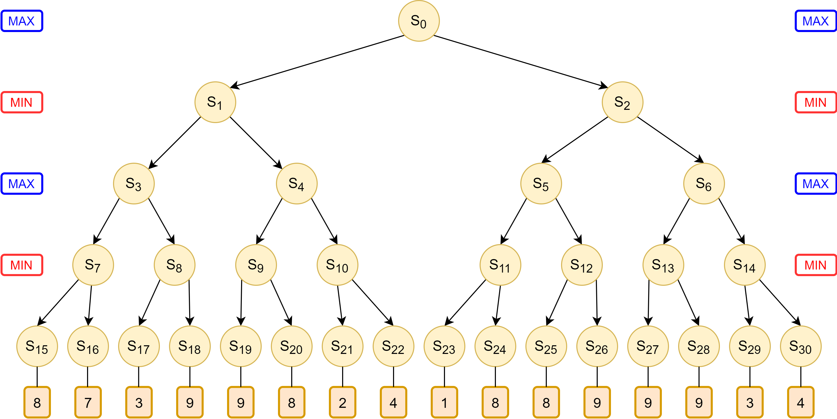
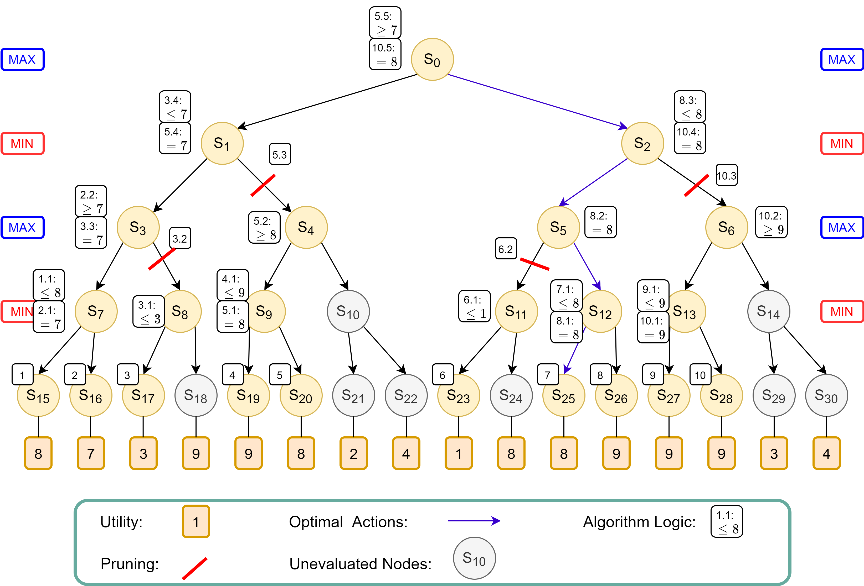
Let us consider the game tree in Figure 4, where MAX player begins first. We will now trace the algorithm’s logic as it processes the game tree, as well as how the algorithm avoids having to evaluate some terminal states.

Figure 4: Game tree where MAX Player starts first.

The algorithm evaluates the nodes from left to right along the game tree recursively. The logic flows in the following order, denoted by the increasing numbers on the white boxes in Figure 5:

• Box 1: The algorithm recursively traverses down from root node $S_0$ to $S_{15}$ to evaluate the first terminal state, which results in a utility of 8
• Box 1.1: The MIN player at $S_7$, knowing that the terminal state at $S_{15}$ will produce utility of 8, now knows that the utility at $S_7$ will be equal to or less than 8, because he could potentially choose $S_{16}$ which might have a lower utility.
• Box 2: The algorithm evaluates the next terminal state $S_{16}$ to find a utility of 7.
• Box 2.1: For the MIN player at $S_7$, the utility of 7 at $S_{16}$ is lower than utility of 8 at $S_{15}$. Thus, he will definitely choose $S_{16}$, and utility at $S_7$ is assigned as 7.
• Box 2.2: The MAX player at $S_3$, knowing that choosing $S_7$ will result in a utility of 7, now knows that his utility will be at least 7, because he can potentially choose $S_8$ that could have a higher utility value.
• Box 3: The algorithm evaluates the next terminal state $S_{17}$ to find a utility of 3.
• Box 3.1: The MIN player at $S_8$, now knows that his utility will be at most 3 from the terminal state $S_{17}$, because he can potentially choose $S_{18}$ which could have a lower utility.
• Box 3.2: The MAX player at $S_3$ now knows that by choosing $S_8$, his utility will be at most 3, which is worse than the option of choosing $S_7$ that gives him utility 7. Thus he will choose $S_7$, and the entire branch to $S_8$ is pruned off, without having to evaluate the remaining nodes.
• Box 3.3: With only $S_7$ remaining, a utility value of 7 is assigned to node $S_3$.
• Box 3.4: The MIN player at $S_1$, knowing that choosing $S_3$ will result in a utility of 7, now knows that the utility at $S_1$ is at most 7, because he can potentially choose $S_{4}$ which could have a lower utility.
• Box 4: The algorithm evaluates the next terminal state $S_{19}$ to find a utility of 9.
• Box 4.1: The MIN player at $S_9$, now knows that his utility will be at most 9 from the terminal state $S_{19}$, because he can potentially choose $S_{20}$ which could have a lower utility.
• Box 5: The algorithm evaluates the next terminal state $S_{20}$ to find a utility of 8.
• Box 5.1: The MIN player at $S_9$ would choose $S_{20}$ which gives a lower utility of 8 compared to $S_{19}$ which gives a utility of 9. Thus the lower utility of 8 is assigned to $S_9$.
• Box 5.2: The MAX player at $S_4$, knowing that choosing $S_9$ results in a utility of 8, knows that his at $S_4$ utility is at least 8 because he could potentially choose $S_{10}$ which might have a higher utility.
• Box 5.3: The MIN player at $S_1$ knows it can pick $S_3$ for utility 7, which is better that picking $S_4$ which grants the utility of at least 8. Therefore, $S_4$ will not be picked, at the entire branch of $S_4$ is pruned.
• Box 5.4: The MIN player at $S_1$ will therefore pick $S_3$ to guarantee a lower utility of 7, thus utility value 7 is assigned to $S_1$.
• Box 5.5: The MAX player at $S_0$, knowing that picking $S_1$ results in a utility of 7, knows that at $S_0$, his utility is at least 7, because he could potentially pick $S_2$ which may have a higher utility.
• Box 6: The algorithm evaluates the next terminal state $S_{23}$ to find a utility of 1.
• Box 6.1: The MIN player at $S_{11}$, knowing that picking $S_{23}$ results in utility 1, now knows that his utility at $S_{11}$ is at most 1, because he can potentially choose $S_{24}$ which may yield a lower utility.
• Box 6.2: The MAX player at $S_5$, knowing that choosing $S_{11}$ will result in a utility at most 1, will not choose $S_{11}$, because he could have chose $S_1$ when he was at $S_0$ and get utility 7. Thus the entire branch of $S_{11}$ is pruned. The utility at is $S_5$ still uncertain as choosing $S_{12}$ could still potentially yield a higher utility than 7.
• Box 7: The algorithm evaluates the next terminal state $S_{25}$ to find a utility of 8.
• Box 7.1: The MIN player at $S_12$, knowing that choosing $S_{25}$ results in a utility of 8, now knows that his utility at $S_{12}$ is at most 8, because he can potentially choose $S_{26}$ which might have a lower utility.
• Box 8: The algorithm evaluates the next terminal state $S_{26}$ to find a utility of 9.
• Box 8.1: The MIN player at $S_{12}$ will choose $S_{25}$ which provides a lower utility of 8. Thus $S_{12}$ is assigned the value of 8.
• Box 8.2: The MAX player at $S_5$ now knows that choosing $S_{12}$ returns a utility of 8, which is higher than the utility of 7 had he chose to choose $S_1$ when he was at $S_0$. Thus, a value of 8 is assigned to $S_5$.
• Box 8.3: The MIN player at $S_2$ knows that choosing $S_5$ results a utility of 8, thus he now knows that the utility at $S_2$ is at most 8, because he can potentially choose $S_6$ which may potential yield a lower utility.
• Box 9: The algorithm evaluates the next terminal state $S_{27}$ to find a utility of 9.
• Box 9.1: The MIN player at $S_13$ knows that choosing $S_{27}$ results in a utility of 9, and now knows that his utility at $S_13$ is at most 9, because he can potentially choose $S_{28}$ which may yield a lower utility.
• Box 10: The algorithm evaluates the next terminal state $S_{28}$ to find a utility of 9.
• Box 10.1: The MIN player at $S_13$ knows that choosing either $S_{27}$ or $S_{28}$ results in a utility of 9, thus assigning a utility of 9 for $S_{13}$.
• Box 10.2: The MAX player at $S_6$ knows that choosing $S_{13}$ results in a utility of 9, thus his utility at $S_6$ is at least 9, because he can potentially choose $S_14$ which may potentially yield a higher utility.
• Box 10.3: The MIN player at $S_2$ knows that choosing $S_6$ results in a utility of at least 9, which is worse than choosing $S_5$ which guarantees a lower utility of 8. Thus, the MIN player will not choose $S_6$, and the entire branch of $S_2$ is pruned.
• Box 10.4: The MIN player at $S_2$ will therefore choose $S_5$ to get a utility of 8. Thus $S_2$ is assigned utility of 8.
• Box 10.5: The MAX player at $S_0$ knows that choosing $S_2$ will result in a utility of 8, which is higher than the utility of 7 by choosing $S_1$. Thus, the MAX player will choose $S_2$ to get a utility of 8 at $S_0$.

Figure 5: Game tree annotated with Alpha-Beta Pruning Logic.

8.2.2. Evaluation of Time/Space Complexity of Alpha-Beta Pruning

One weakness of the Alpha-Beta pruning algorithm is that it is sensitive to the order in which the terminal states are evaluated. If the algorithm happens to evaluate the worse successors first in all nodes, there would be no chance for optimization by pruning.

Therefore in the worst case, the algorithm runs the same as the Minimax Search with $O(b^m)$ time complexity. However, if the algorithm knows where to prioritize the search of the best successor nodes first, it only needs to examine $b^{m/2}$ nodes, and therefore improves its time complexity to $O(b^{m/2})$ in the best case. If the successors are evaluated randomly, the algorithm’s time complexity becomes $O(b^{3m/4})$ on average. The space complexity is similar to that of the Minimax algorithm.

8.3. Heuristic Function for Imperfect Decision-Making

Because Alpha-beta pruning still has to explore the game tree until the terminal state, this makes its time complexity impractical in games with large depth such as chess. One strategy is to cut off the search earlier, and apply a heuristic evaluation function to each state at the cutoff, thus allowing for non-terminal nodes to become leaves of the smaller search tree.

A good heuristic evaluation function should have the following properties:

1. The evaluation function should evaluate terminal states in a similar preference order as the true utility function would on the terminal states.

2. Computation of the evaluation function should not take too long (ideally close to constant time complexity)

3. For non-terminal states, the evaluation function should choose states highly correlated with the chances of winning. The uncertainty is induced by computational limits.

For example in chess, an evaluation function the expected probability of a win based on a weighted linear function of certain features of the game. For example, the evaluation function can be, \(EVAL(S)=w_1 f_1(S)+w_2 f_2(S)+\cdots +w_n f_n(S)\) where $w_i$ refers to the weights, while $f_i(S)$ refers to a computation of features in the game state, such as the number of a type of chess piece on the board. The evaluation function need not calculate the actual probability of winning, but the ordinal relation between states via the evaluation function should be similar to that of the expected probability of winning.

The Alpha-beta pruning algorithm could implement the cut-off and heuristic by modifying the terminal condition of the algorithm.

Algorithm 7 MinimaxDecision($S$)

1. $bestAction \leftarrow null$
2. $max \leftarrow -\infty$
3. for all action $a$ in ACTIONS$(S)$ do
4. $~~~~~$ $util \leftarrow$ MinValue(RESULT($S$,$a$), $1$, $max$, $\infty$)
5. $~~~~~$ if $util > max$ then
6. $~~~~~~~~~~$ $bestAction \leftarrow a$
7. $~~~~~~~~~~$ $max \leftarrow util$
8. return $bestAction$

Algorithm 8 MinValue($S$, $depth$, $\alpha$, $\beta$)

1. if CUTOFFTEST($S, depth$)=True then return EVAL($S$)
2. $v \leftarrow \infty$
3. for all action $a$ in ACTIONS($S$) do
4. $~~~~~$ $v \leftarrow$ min($v$, MaxValue(RESULT($S$,$a$), $depth+1$, $\alpha$, $\beta$))
5. $~~~~~$ if $v \leq \alpha$ then return $v$
6. $~~~~~$ $\beta \leftarrow$ min($v,\beta$)
7. return $v$

Algorithm 9 MaxValue($S$, $depth$, $\alpha$, $\beta$)

1. if CUTOFFTEST($S, depth$)=True then return EVAL($S$)
2. $v \leftarrow -\infty$
3. for all action $a$ in ACTIONS($S$) do
4. $~~~~~$ $v \leftarrow$ max($v$, MinValue(RESULT($S$,$a$), $depth+1$, $\alpha$, $\beta$))
5. $~~~~~$ if $v \geq \beta$ then return $v$ $\text{// Pruning of branch}$
6. $~~~~~$ $\alpha \leftarrow$ max($\alpha,v$)
7. return $v$

One way to control the amount of search is to set a depth limit $d$ so that CUTOFFTEST($S, depth$) returns true when depth reaches limit $d$ or a terminal state is reached whichever is earlier. The depth limit can be determined by the deepest depth a computer can explore while just keeping to the time limit required to make a decision. With a cut-off, the time complexity improves to $O(b^{3d/4})$ on average where $d<m$ .