Chapter 5 Constraint Satisfaction Problem

Constraint Satisfaction Problems (CSP) uses a factored representation of each state, with each state associated with a set of variables(X), each variable containing a value from its domain(D). The objective of the problem to find the value for each of the variable that satisfy all the constraints(C) of the problem.

A CSP comprise of three components:

Set of variables: $X$: { $x_1, x_2, \ldots , x_n$}
Set of domains(D) belonging to each variable { $D_1, D_2, \ldots , D_n$ } where $D_i=domain(x_i)$
Set of constraints(C) that specifies the valid combinations of values assigned to each of the variable.

In CSP the order of series of action has no effect on possible outcome, hence CSP problems are commutative. Let us consider an algorithm to solve CSP.

Backtracking Search

One useful algorithm to solve CSP is the Backtracking Search. Let us try to represent 4-Queen puzzle as CSP, for that first we have to find variable, possible domain for each of the variable, and constraint to solve.

We can describe the CSP as follows:

Variables: { $x_1, x_2, x_3, x_4$}, where each $x_i$ represent the variable for $i^{th}$ column in $4 \times 4$ grid.
For each variable $x_i$: $D_{x_i}$={$1,2,3,4$}, $D_{x_i}$ represent the value of the row, i.e. each variable $x_i$ can possibly take a value of the row.
Constraints: Let NOATTACK($x_i,x_j$) return True if the queen at $x_i$ cannot attack the queen at $x_j$, and False otherwise.
1. NOATTACK($x_1,x_2$)
2. NOATTACK($x_1,x_3$)
3. NOATTACK($x_1,x_4$)
4. NOATTACK($x_2,x_3$)
5. NOATTACK($x_2,x_4$)
6. NOATTACK($x_3,x_4$)

We can specify the constraints fully for each NOATTACK($x_i,x_j$) in a huge truth table as seen in Table below:

Specifying constraints on a huge truth table
$x_1$	$x_2$	NOATTACK
1	1	False
1	2	False
1	3	True
1	4	True
2	1	False
...	...	...

Our goal is to choose the values of all $x$ so that none of the queens in their respective positions can attack each other.

Backtracking Search Algorithm

We first consider a naive algorithm that does not check for consistency of the variables in the process of assigning values to them. Algorithm 1 represents the naive Backtracking approach for CSP.

Algorithm 1 BacktrackingSearch(prob,assign)

If AllVarsAssigned(prob,assign) then
$~~~~~$If IsConsistent(assign) then
$~~~~~~~~~~$ Return assign
$~~~~~$Else
$~~~~~~~~~~$ Return failure
var$\gets$PickUnassignedVar(prob,assign)
For value$\in$ OrderDomainValue(var,prob,assign) Do
$~~~~~$ assign$\gets$ assign $\cup$ (var = value)
$~~~~~$ result $\gets$ BacktrackingSearch(prob,assign)
$~~~~~$If result != failure then Return result
$~~~~~$ assign $\gets$ assign $\setminus$ (var=value)
Return failure

Let us try to execute the Algorithm 1 step by step for 4-Queen puzzle. Figure 1 represents the board overview of backtracking algorithm to solve 4-Queen puzzle.


*Figure 1: Board state at various steps of naive Backtracking Search.*

Let be the $i^{th}$ functional call, and $j^{th}$ operation in that functional call. The execution of the algorithm goes as follows:

1.1 Pick variable $x_1$; 1.2 Set $x_1=1$
2.1 Pick variable $x_2$; 2.2 Set $x_2=1$
3.1 Pick variable $x_3$; 3.2 Set $x_3=1$
4.1 Pick variable $x_4$; 4.2 Set $x_4=1$
5.1 IsConsistent(assign)=False, thus back track; 4.3 Set $x_4=2$
5.1 IsConsistent(assign)=False, thus back track; 4.4 Set $x_4=3$
5.1 IsConsistent(assign)=False, thus back track; 4.5 Set $x_4=4$
5.1 IsConsistent(assign)=False, thus back track
4.6 Finished ‘for’ loop, thus back track; 3.3 Set $x_3=2$
4.1 Pick variable $x_4$; 4.2 Set $x_4=1$
5.1 IsConsistent(assign)=False, thus back track; 4.3 Set $x_4=2$
5.1IsConsistent(assign)=False, thus back track; 4.4 Set $x_4=3$
5.1 IsConsistent(assign)=False, thus back track; 4.5 Set $x_4=4$
5.1 IsConsistent(assign)=False, thus back track
4.6Finished ‘for’ loop, thus back track
$\cdots$

As shown in the above execution of the Algorithm 1 for 4-Queen puzzle, the main drawback of the algorithm is to check at the end if the assignment is consistent or not. It assigns a possible value to each of the four variables, and then check at the end if the assignment is consistent, and if not, algorithm changes the value of one of the variable and repeat again. Therefore, Algorithm 1 would simply check for consistency with respect to all possible permutation of values $1$ to $4$ assigned to each of the four variables $x_1$ to $x_4$.

Improved Backtracking Search

To overcome the issue of Algorithm 1 , a better approach would be every time the algorithm has to assign a value to a variable, it first checks to ensure that the assigned value is consistent with the previous assignments. Therefore, the improved Algorithm 2 assigns a position to the queen only if it can not be attacked by other queen.

Algorithm 2 BacktrackingSearch(prob,assign)

If AllVarsAssigned(prob,assign) then
var$\gets$PickUnassignedVar(prob,assign)
For value$\in$ OrderDomainValue(var,prob,assign) Do
$~~~~~~~$If ValIsConsistentWithAssignment(value,assign) then
$~~~~~~~~~~~~~~$ assign$\gets$ assign $\cup$ (var = value)
$~~~~~~~~~~~~~~$ result $\gets$ BacktrackingSearch(prob,assign)
$~~~~~~~~~~~~~~$If result != failure then Return result
$~~~~~~~~~~~~~~$ assign $\gets$ assign $\setminus$ (var=value)
Return failure

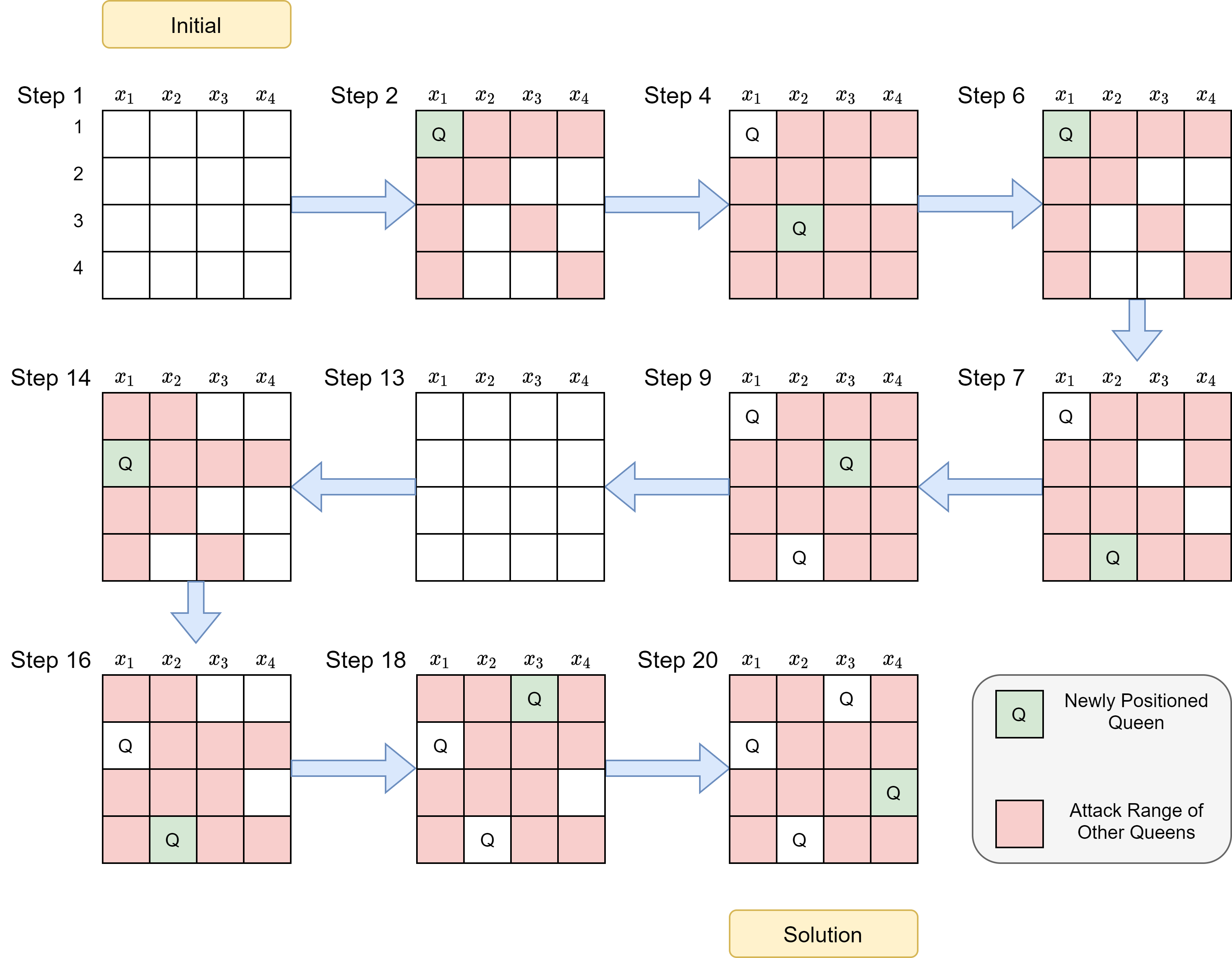
Let us try to execute the Algorithm 2 step by step for 4-Queen puzzle. Figure 2 represents the board overview of backtracking algorithm to solve 4-Queen puzzle.


*Figure 2: Board state at various steps of improved BacktrackingSearch*

The execution of the algorithm goes as follows:

1.1 Pick $x_1$; 1.2 Set $x_1=1$
2.1 Pick $x_2$; 2.2 Set $x_2=3$ as ${1,2}$ is attackable
3.1 Pick $x_3$; Return $failure$ as $ {1,2,3,4}$ are attackable
2.3 Set $x_1=4$ as $ {1,2}$ is attackable and ${3}$ had been assigned
3.1 Pick $x_3$; 3.2 Set $x_3=2$ as $ {1,3,4}$ are attackable
4.1 Pick $x_4$
4.2 Return $failure$ as $ {1,2,3,4}$ are attackable
3.3 Return $failure$ as $ {1,3,4}$ are attackable and ${2}$ had been assigned
2.4 Return $failure$ as $ {1,2}$ are attackable and ${3,4}$ had been assigned
1.3 Set $x_1=2$
2.1 Pick $x_2$; 2.2 Set $x_2=4$ as $ {1,2,3}$ are attackable
3.1 Pick $x_3$; 3.2 Set $x_3=1$ as $ {2,3,4}$ are attackable
4.1 Pick $x_4$; 4.2 Set $x_4=3$ as $ {1,2,4}$ are attackable
5.1 Return $assign$ because all variables are assigned

As seen from the execution of the Algorithm 2 , checking consistency every time a value is assigned to variable improves the efficiency, and we reach goal state in less number of steps than with Algorithm 1.

Backtracking Search with Inference

An another idea to improve the efficiency of the Backtracking Search is that once the algorithm assigns a value to a variable $x_i$, it checks for all the constraints that $x_i$ appears to infer the restrictions on rest of the variables and avoid picking values that are not consistent with previous assignments and possible future assignments.

We have a new function Infer($prob,var,assign$), that output a set of assignments that can be inferred based on the constraints of the problem, whenever a $value$ is assigned to variable. If it is inferred that we can not assign a value to all variables consistently, the function returns a $failure$. In other words, the function helps to make inferences on what values other unassigned variables can take. In CSPs, assigning a value to a variable could lead to restrictions the value that other variables can take, which in turn could propagate the restrictions to other variables. Infer function aims to identify these restrictions and to use them to further restrict the search space.

Algorithm 3 represents the improved backtrack algorithm with inference.

Algorithm 3 BacktrackingSearch_with_Inference(prob,assign)

If AllVarsAssigned(prob,assign) then
var$\gets$PickUnassignedVar(prob,assign)
For value$\in$ OrderDomainValue(var,prob,assign) Do
$~~~~~~~$If ValIsConsistentWithAssignment(value,assign) then
$~~~~~~~~~~~~~~$ assign$\gets$ assign $\cup$ (var = value)
$~~~~~~~~~~~~~~$ inference$\gets$ Infer(var,prob,assign)
$~~~~~~~~~~~~~~$ assign$\gets$ assign $\cup$ inference
$~~~~~~~~~~~~~~$ If inference != failure then
$~~~~~~~~~~~~~~~~~~~~~~~~$ result $\gets$ BacktrackingSearch(prob,assign)
$~~~~~~~~~~~~~~~~~~~~~~~~$If result != failure then Return result
$~~~~~~~~~~~~~~$ assign $\gets$ assign $\setminus$ {(var=value) $\cup$ inference
Return Failure

Below is the execution of Algorithm3 for $4-Queen$ problem:

1.1 Pick $x_1$; 1.2 Set $x_1=1$
1.3 $inference$ returned as $failure$, remove assignment $x_1=1$
1.4 Set $x_1=2$
1.5 $inference$ returned as ${x_2=4, x_3=1, x_4=3}$
2.1 Return $assign$ because all variables are assigned

Inference Function Logic at Step 3

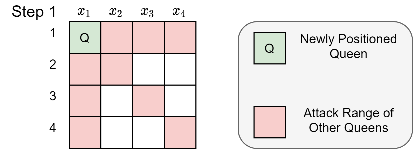
At step 3, because $x_1=1$, the inference function is able to deduce that the red squares in the Figure 3 are within a queens attacking range and no other queens can be placed there.


*Figure 3: Board state at various steps of improved BacktrackingSearch with Inference*

Then, the inference function looks at each and every constraint to infer restrictions on rest of the variables.

Constraint 1:NOATTACK($x_1,x_2$)
- Observation from Figure 3: $x_1=1 \Rightarrow x_2 \notin {1,2}$
Constraint 2:NOATTACK($x_1,x_3$)
- Observation from Figure 3: $x_1=1 \Rightarrow x_3 \notin {1,3}$
Constraint 3:NOATTACK($x_1,x_4$)
- Observation from Figure 3: $x_1=1 \Rightarrow x_4 \notin {1,4}$
Constraint 4:NOATTACK($x_2,x_4$)
- Because $x_2 \in {3,4}$,
- If $x_2=3 \Rightarrow x_4=2$
- If $x_2=4 \Rightarrow x_4=3$
Constraint 5:NOATTACK($x_2,x_3$)
- Deduction: $x_2 \in {3,4} \Rightarrow x_3 \notin {3,4}$
- Deduction: $x_3 \notin {3,4} \wedge x_3 \notin {1,3} \Rightarrow x_3 \notin {1,3,4} \Rightarrow x_3=2$
Constraint 6:NOATTACK($x_3,x_4$)
- Deduction: $x_3=2 \Rightarrow x_4 \notin {1,2,3}$
- Deduction: $x_4 \notin {1,2,3} \wedge x_4 \notin {1,4} \Rightarrow x_4 \notin {1,2,3,4}$
- Therefore,with no possible value to assign to $x_4$, $x_1=1$ is not going to work as a solution, return failure and backtrack

Inference Function Logic at Step 5

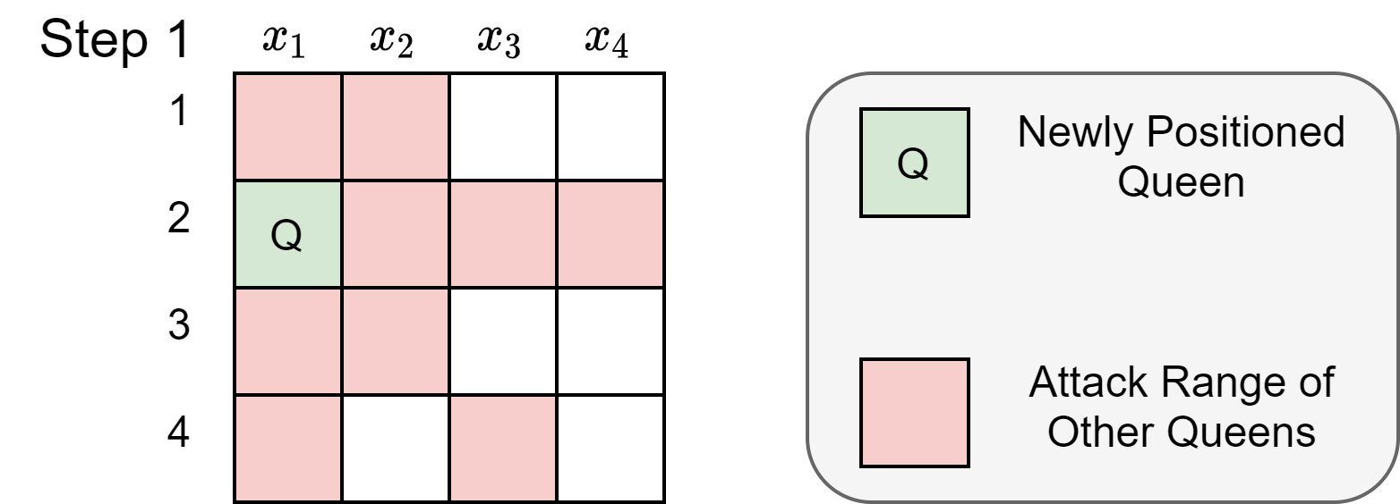
At step 5, because $x_1=2$, the inference function is able to deduce that the red squares in the Figure 4 are within a queens attacking range and no other queens can be placed there.


*Figure 4: Board state at various steps of improved BacktrackingSearch with Inference*

Then, the inference function looks at each and every constraint to infer restrictions on rest of the variables.

Constraint 1:NOATTACK($x_1,x_2$)
- Observation from Figure 4 : $x_1=2 \Rightarrow x_2 \notin {1,2,3} \Rightarrow x_2=4$
Constraint 2:NOATTACK($x_1,x_3$)
- Observation from 4: $x_1=2 \Rightarrow x_3 \notin {2,4}$
Constraint 3:NOATTACK($x_1,x_4$)
- Observation from 4: $x_1=2 \Rightarrow x_4 \notin {2}$
Constraint 4:NOATTACK($x_2,x_4$)
- Deduction: $x_2=4 \Rightarrow x_4 \notin {2,4}$
- Deduction: $x_4 \notin {2,4} \wedge x_4 \notin {4} \Rightarrow x_4 \notin {2,4}$
Constraint 5:NOATTACK($x_2,x_3$)
- Deduction: $x_2=4 \Rightarrow x_3 \notin {3,4}$
- Deduction: $x_3 \notin {3,4} \wedge x_3 \notin {2,4} \Rightarrow x_3 \notin {2,3,4} \Rightarrow x_3=1$
Constraint 6:NOATTACK($x_3,x_4$)
- Deduction: $x_3=1 \Rightarrow x_4 \notin {1,2}$
- Deduction: $x_4 \notin {1,2} \wedge x_4 \notin {2,4} \Rightarrow x_4 \notin {1,2,4} \Rightarrow x_4=3$
- Therefore,the function returns ${x_2=4, x_3=1, x_4=3}$

The Backtracking search with an inference function, Algorithm 3, therefore becomes much more efficient. The overall efficiency however, is now strongly dependent on the efficiency of the Infer function which can be very costly to implement.

Now, the important question is How to implement the Infer functions? Let us discuss important questions related to functions:

Representation of data-structure: It stores each of the variable $x_i$, and set of values that $x_i$ is not supposed to take, such a set of values grows as Infer makes deductions based on the current assignment and constraints. For example: $x_1 \notin{1,2}, x_2 \notin {1,3,4}\ldots$

Store the constraints: The naive approach to store the constraints could be storing them as a truth-table described in Table 1, but we know that it is not efficient to use truth-tables for larger data; hence the more efficient way of storing the constraints is to come-up with some function that can returns true/false depending on the current values of the argument variables. Definitions of such a function depend on the application, for example for $n-Queen$ problem, such a function can be $f(x_1,x_2) { if {|val(x_1)-val(x_2)| > 1} \; \text{return True else False} }$.

ComputeDomain($\boldsymbol{x,assign,inference}$):In addition to above discussed questions, we also need an way to compute the domain of a variable x given an assignment and inference. We use a function ComputeDomain$(x,assign,inference)$ to return the domain of variable x given assignment and inference. Again, the definition of ComputeDomain function is not fixed and mainly depends on the application and inference definition. For example: if we have the assignment, ${x_1 = 1}$ and the inference, ${x_1 \notin {2,3}}$, then the ComputeDomain${(x_1,assign,inference)}$ should output the domain of $x_1$ as ${1}$. In another example for the assignment, ${x_2 = 1}$ and the inference, ${x_1 \notin {2,3}}$ the ComputeDomain${(x_1,assign,inference)}$ should output the domain of $x_1$ as ${1,4}$.>

Algorithm 4 represents function of Algorithm 3.

Algorithm 4 Infer(prob,var,assign) function of Algorithm 3

inference $\gets \emptyset$
varQueue $\gets$ [var]
While varQueue is not empty Do
$~~~~~~~$ y $\gets$ varQueue.pop()
$~~~~~~~$ For each constraint C in prob where y $\in$ Vars(C) Do
$~~~~~~~~~~~~~$ For all x $\in$ Vars(C)$\setminus$y Do
$~~~~~~~~~~~~~~~~~~~~~$ S $\gets$ ComputeDomain(x,assign,inference)
$~~~~~~~~~~~~~~~~~~~~~$ For each value v $\in$ S Do
$~~~~~~~~~~~~~~~~~~~~~~~~~~~$ If no valid value exists $\forall$ var $\in$ Vars(C)$\setminus$ x s.t. C[x $\vdash$ v] is satisfied then
$~~~~~~~~~~~~~~~~~~~~~~~~~~~~~~~~~~~$ inference $\gets$ inference $\cup$ (x $\not \in {v})
$~~~~~~~~~~~~~~~~~~~~$ T $\gets$ ComputeDomain(x,assign,inference)
$~~~~~~~~~~~~~~~~~~~~$ If T $= \emptyset$ then Return faliure
$~~~~~~~~~~~~~~~~~~~~$ IF S $\neq$ T then varQueue.add(x)
Return inference

Example in N-queen problem

Recall in the N-queen problem for Algorithm 4, at the start of the execution of the algorithm, the assignment $x_1=1$ was made and the inference function is then called on this assignment.

$x_1$ is pushed and popped, and all the constraints in the problem involving variable $x_1$ is iterated over a for loop, namely: NOATTACK($x_1,x_2$),NOATTACK($x_1,x_3$),NOATTACK($x_1,x_4$).

For the first constraint NOATTACK($x_1,x_2$) to be iterated, the inner for loop calls upon $x$ in the constraint that is not $x_1$, which in this case is only $x_2$. The initial domain for $x_2$ stored in $S$ is $\{1,2,3,4\}$. For each value in $S$, we check if there is a valid value for $x_2$ so that NOATTACK($x_1,x_2$) is satisfied. In this case the domain of $x_1$ is $1$ because it has already been assigned that value. For example, when $x_2=2$, no valid value for $x_1\in \{1\}$ exists so that the constraint is satisfied, therefore, $x_2\notin \{1\}$ is added into inference. The same is done $x_2=2$ and $x_2\notin \{2\}$ is added to inference. However, there are no inconsistencies for $x_2\in{3,4}$ so those are not added into inference. After that, the domain for $x_2$ is computed again with the updated inference, which returns set $T$ as $x_2\in\{3,4\}$, which is not an empty set, but is also not the same as $S$. Thus, $x_2$ is added into $varQueue$.

The same process is iterated for the other remaining constraints to add in values of $x_3$ and $x_4$ into $inference$.

When $x_2$ is popped from the $varQueue$, all the constraints in the problem involving variable $x_2$ is iterated over a for loop, namely: NOATTACK($x_1,x_2$), NOATTACK($x_2,x_3$), NOATTACK($x_2,x_4$).

For example sake, let us consider constraint NOATTACK($x_2,x_3$). The inner for loop then calls upon $x$ in the constraint that is not $x_2$, which in this case is only $x_3$. The initial domain for $x_3$ stored in $S$ is $\{2,4\}$. For each value in $S$, we check if there is a valid value for $x_3$ so that NOATTACK($x_2,x_3$) is satisfied. For example, when $x_3=4$, no valid value of $x_2\in \{3,4\}$ exists so that NOATTACK($x_2,x_3$) is satisfied, so $x_3\notin \{4\}$ is added into the constraint. However, $x_3=4$ has no inconsistencies so it is not added into inference. After that, the domain for $x_3$ is computed again with the updated inference, which returns $T$ as $x_3\in\{2\}$, which is not an empty set, but is also not the same as $S$. Thus, $x_3$ is added into $varQueue$.

The algorithm continues on until it reaches constraint NOATTACK($x_3,x_4$), where the $T$ for $x_4$ is am empty set, thus returning failure to the main backtracking algorithm.

Alternative Implementation of Inference

The computation required for Infer function can be expensive, and may potentially slow down the search. Some alternative implementation attempts to limit the depth of the inference in order to reduce computational cost. However, one important point to note here is this would also mean that the backtracking algorithm does not benefit from information that can be derived from deeper levels of inference.

The alternative implementations are as follows:

Don’t add any variable to $varQueue$ at each iteration. This is the equivalent of deleting Line 13 of the Algorithm4.
1. This ensures that the inference will rule out only some of the values of variable.
2. This variant of inference is also known as Forward Checking.
3. Although forward checking can rule out many inconsistencies, it does not infer further ahead to ensure arc consistency for all the other variables.
Replace the $S\neq T$ condition in Line 13, replace with $|T|=1$.
1. This goes one step further from forward checking, and allows for further inferences for the variables that have one valid value in the domain.
2. Depending on the complexity of the application, the condition can be set to any particular value, e.g $|T|\leq 3$.

In addition to aforementioned different variants of implementation, there are many heuristics that are proved to efficient in backtracking-search algorithms.

Minimum Remaining Value Heuristic: In PickUnassignedVar function of the backtracking search always choose the next unassigned variable that have the smallest domain size. The idea behind this heuristic is to assign values to variables that is most likely to cause failure quickly, thus allowing for pruning of larger branches in the search tree.

Least Constraining Value Heuristic: In OrderDomainValue function of the backtracking search always pick a value in the domain that rules out the least domain values of other neighboring variables in the constraint. This allows for the maximum flexibility for subsequent variable assignments. This heuristic is only relevant if we are interested in a single solution. If we want to find all (multiple) solutions to the problem, then the all values for an assignment to a variable will be iterated through in any case, thus it is not relevant here.

How Hard is Constraint Satisfaction Problem?

Nevertheless, the ways described are only heuristics and not guaranteed to perform well in any kind of problem. In fact, CSPs are very hard to solve, belonging to a set of problems known in Computer Science as NP-Complete where there are no Polynomial time solutions to solve these problems but the answer to these problems can be checked in polynomial time. There are multiple variants of CSPs, and while most are NP-Complete, some can be solved in Polynomial time. Below lists some of the variants of CSPs.

There are some special variants of CSP as listed below:

Binary CSP: Every constraint is defined over two variables(NP-complete).
Boolean CSP(SAT): The domain of every variable is 0,1(NP-complete).
2-SAT: Combination of Binary CSP and Boolean CSP, that is, every constraint is defined over two variables and the domain of every variable is 0,1(Polynomial time(P)-solvable).