Chapter 4
Local Search and Optimization Problems
The problems covered so far dealt with agents having to choose a series of actions to reach the goal state, where the path to the goal constituted the solution to the problem. In some other problems, the path to the goal is irrelevant as only the end state is required for the solution.
An example would the $n$-Queen puzzle. We are given an $n×n$ chess board and $n$ chess queens which travel vertically, horizontally and diagonally to attack. The $n$-Queen puzzle asks us to find a configuration of the queens on the board such that none of the queens can attack each other in one move?
Suppose we are given the $4\times 4$ chess board as in Figure 1 (left). The initial board is clearly not the solution because each queen can attack other queens diagonally. How can we design and algorithm that will lead to the solution board on the right?
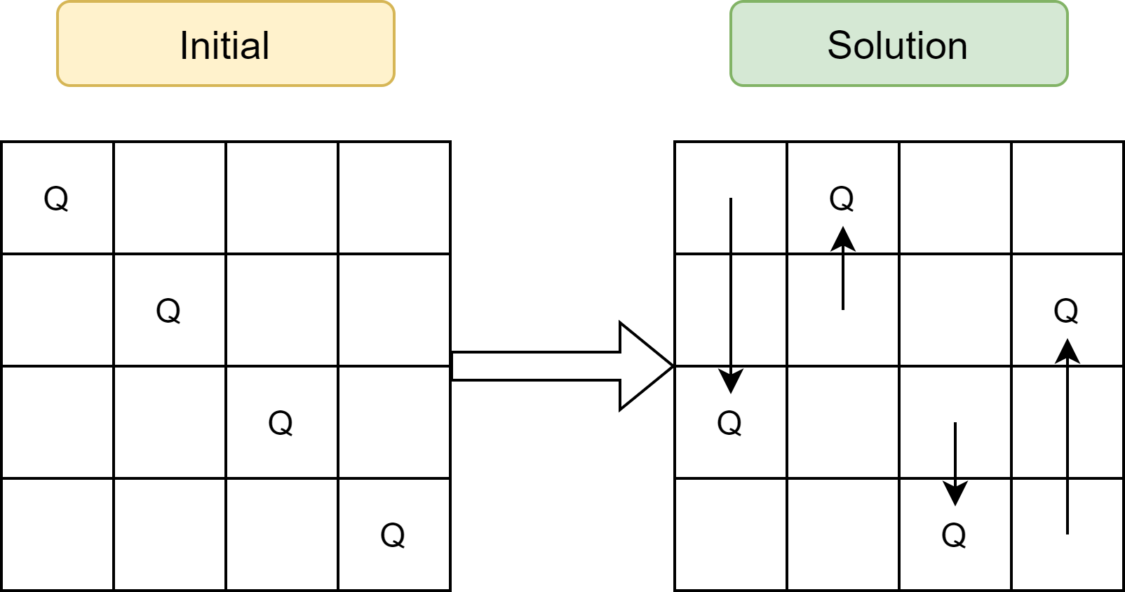 |
|---|
| Figure 1: 4×4 Boards with 4 Queens |
One way to break down the problem is to restrict the transition of one board state to another to the movement of queens across rows (i.e. along the columns) because we already have one queen in each column. This means board can transition to another state by moving up and down. The new abstracted problem can be broken down as follows:
- $S$ : The set of board states with queens at various positions.
- $N(S)$ : Neighbors of a state $S$, i.e. the set of new board states brought about by an action such as moving the queen.
- $val(S)$ : Value of a state. The value should reflect the notion of ‘quality’ of a state, in a sense of how close it is to the goal state. Naturally $val(S) = 0$. For $n$-Queens, $val(S)$ is the number of pairs of queens that can attack each other.
Hill-Climbing Search Algorithm
A useful way to find the solution is to run the Hill-Climbing Search algorithm. Hill-Climbing Search is a loop that continually moves the game state to an increasing (or decreasing) value until it reaches a local ‘peak’. It does not look beyond the immediate neighboring states, and does not remember past states.
Algorithm 1 $HillClimb(S)$
- $minVal \leftarrow $ $val(S)$
- $minState \leftarrow $ { } $~~~~~~~~~~~~~~~~~~$ //Only 1 thing to track
- for each $u$ in $N(S)$ do
- $~~~~~$ if $val(u)<minVal$ then
- $~~~~~~~~~~$ $minVal = val(u)$
- $~~~~~~~~~~$ $minState = u$
- return $minState$
Algorithm 2 $SolveNQueens(initialState)$
- $S \leftarrow initialState$
- while $val(S)!=0$ do
- $~~~~~~$ $S \leftarrow HillClimb(S) $
- return $S$
A weakness in Hill-Climbing Search
One weakness of the Hill-Climbing algorithm is that it greedily chooses the neighboring state that has a better value. However, at times there are occasions where in order to reach the solution, the state has to transition to a slightly worse value first. For example in Figure 2, the board state has to transition
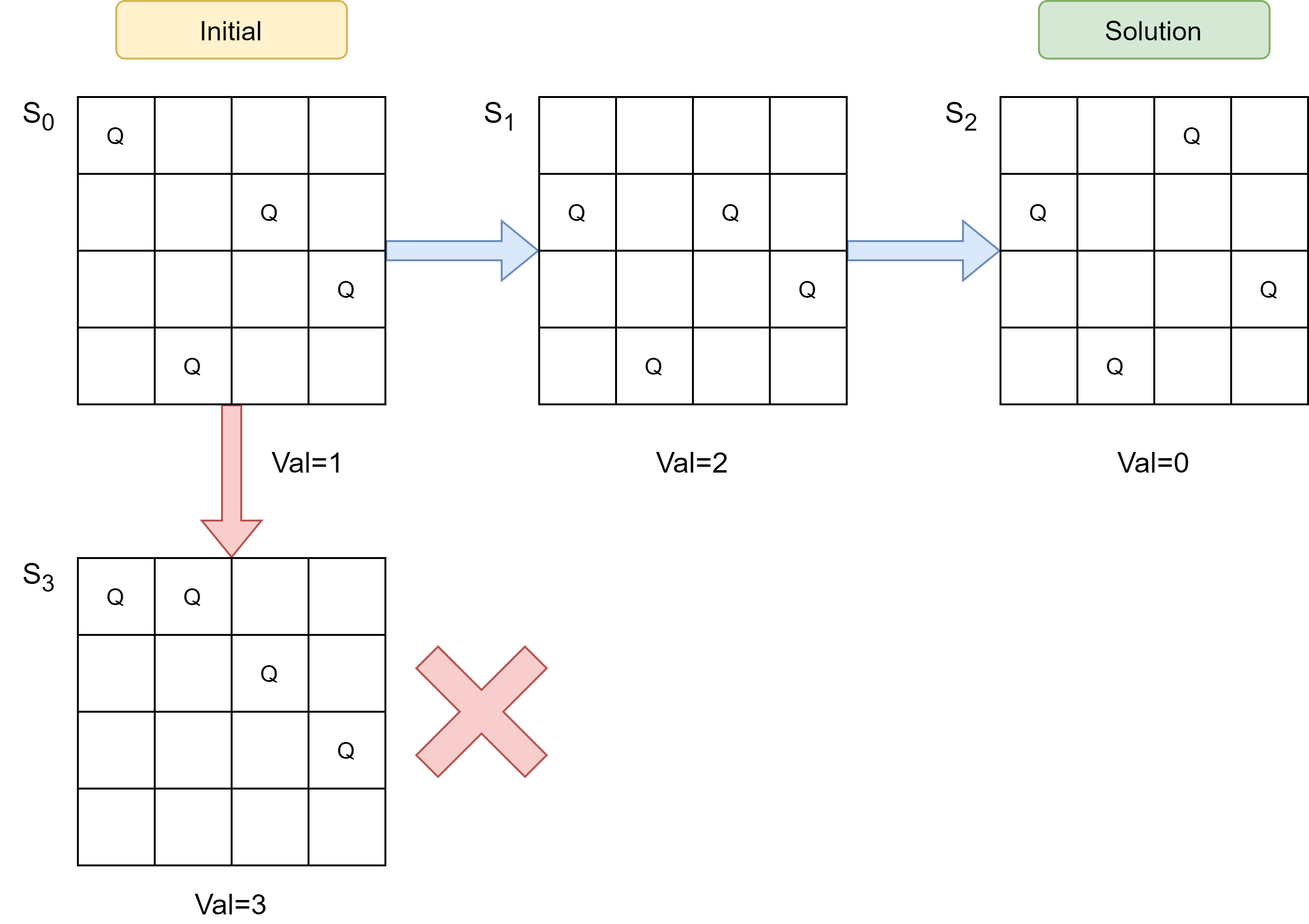 |
|---|
| Figure 2: Board state having to transition to higher value to reach solution |
from initial state $S_0$ with a value of 1 to state $S_1$ with a worse value of 2, before it can reach the solution $S_2$ with a value of 0. Thus a more ideal algorithm would allow for a state transition that worsens the state value occasionally. However, this allowance of state transition to a worse state value should be weighed against some form of preference that would lead to the right solution. As seen from a transition of initial state to state $S_3$ , the value worsened to 3, but the board is further away from the solution.
Simulated Annealing
As we already discussed that Hill-Climbing has an issue of getting stuck at local minimum/maximum. One of possible way to over this issue is to allow mistake sometimes; allowing mistake is to allow to choose neighbor that have lower(resp. higher) value than the current state, and that might not be the ideal move to achieve minimum (resp. maximum). One such algorithm, that allows us to make mistakes is Simulated Annealing. Simulated Annealing is inspired by the process in metallurgy where metals and glasses are hardened by heating them to high temperature and then cooling them down gradually (based on a cooling schedule) so that the material hardens into a low-energy crystalline structure. In condensed-matter, we have a type of spin models, i.e we have atoms and all of them have spin either $+1$ or $−1$ with equal probability. Let us assume $μ_i$ is the spin of atom $i$, then the $\Pr[μ_i= 1] = \frac{1}{2}$, and the energy of the system $C$ is given by:
\[E(C) = exp\left( - \frac{\underset{(i,j) \in N}{\sum}J\mu_i\mu_j}{K_BT} \right)\]where $T$ is the temperature and $K_B$ is the Boltzman constant. At normal temperature, we have on an average half of the atoms labeled $−1$, and another half as $+1$. Our objective here is to achieve a state with lowest energy. A state $C$ is at lowest energy, if all the atoms at state C have spin $+1$ or $−1$. The probability of moving a state $C_a$ to $C_b$:
\[\Pr[C_a \rightarrow C_b] \propto exp\left({\frac{E(C_a) - E(C_b)}{K_BT}}\right)\]Now, at this point, the question is How can we get into the lowest energy state. The procedure is, first have the high temperature and then slowly decrease the temperature. How the material scientists facilitate the transition of a configuration to a lower energy state is through the cooling schedule. The cooling schedule is given by the function that outputs the temperature $T$, and is a decreasing function of time. As a result, at the beginning when temperature is high, the configuration easily moves with a high probability even when $E(C_b) > E(C_a)$. As time goes on and the temperature falls, the $\Pr[C_a→ C_b]$ starts to decline. So basically, at the start, we allow atoms to transfer to the high energy state in order to finally achieve global minimum energy state.
Algorithm 3 describes the process of simulated annealing to achieve global minimum. The $Schedule$ function typically decreases with time but it is always up to the user to define the function on how gradual the simulated annealing process should be.
Algorithm 3 SimulatedAnnealing$(initialState)$
- $C \leftarrow initialState$
- for $t = 0$ to $\infty$ do
- $~~~~~$ $C’ \leftarrow PickRandomNeighbour(C)$
- $~~~~~$ $T \leftarrow Schedule(t) ~~~~~~~~~~~~~~~~~~$ //Assume that $val(Goal) = 0$
- $~~~~~$ if $val(C’) = 0$ then
- $~~~~~~~~~~$ return $C’$
- $~~~~~$ if $val(C’) < val(C)$ then
- $~~~~~~~~~~$ $C \leftarrow C’$
- $~~~~~$ else
- $~~~~~~~~~~$ $C \leftarrow C’$ with Probability $\propto exp\left( \frac{val(C)-val(C’)}{K_BT}\right)$
In Algorithm 3, we terminate when $val(C’)$, but for some cases, the $val(Goal)$ may not be defined. Such a problem can be seen as an optimization problem to minimize the value of solution state.
We can then define the $Schedule$ function to return 0 value based on certain criteria or after a finite number of iterations or modify the terminating criteria as per the application.
The idea of simulated annealing works well in practice, but it is not guaranteed to achieve global minima in every case. Hence, like hill-climbing, simulated annealing is also not complete.