Informed Search

3.1 A* Algorithm

The key idea of A* algorithm comes from Uniform Cost Search. A* is same as UCS except that it has extra knowledge that can guide the search, which is known as a heuristic $h(n)$. $h(n)$ is an estimate of the cost of the shortest path from node $n$ to a goal node, and we have to compute $h(n)$ also. For a time being, let us assume that we know $h(n)$ for all the nodes, later we will discuss in detail about how to compute such heuristics. $A^{*}$ search evaluates nodes using an estimated cost of the optimal solution, therefore

Algorithm 6 A* Algorithm: FindPathToGoal($u$)

1. $F$(Frontier) $\leftarrow$ PriorityQueue($u$) $~~~~~~~~~~~~~~$ // This should be implemented with $\hat{f}$ minimum
2. $E$(Explored) $\leftarrow$ $ \{ u \} $
3. $\hat{g}[u] \leftarrow 0$
4. while $F$ is not empty do
5. $~~~~~$ $u \leftarrow F$.pop()
6. $~~~~~$ if GoalTest $(u)$ then
7. $~~~~~~~~~~$ return path $(u)$
8. $~~~~~$ $E$.add $(u)$
9. $~~~~~$ for all children $v$ of $u$ do
10. $~~~~~~~~~~$ if $v$ not in $E$ then
11. $~~~~~~~~~~~~~~~$ if $v$ in $F$ then
12. $~~~~~~~~~~~~~~~~~~~~$ $\hat{g}[v] = min(\hat{g}[v],\hat{g}[u]+c(u,v))$
13. $~~~~~~~~~~~~~~~~~~~~$ $\hat{f}[v] = h[v] + \hat{g}[v]$
14. $~~~~~~~~~~~~~~~$ else
15. $~~~~~~~~~~~~~~~~~~~~$ $F$.push(v)
16. $~~~~~~~~~~~~~~~~~~~~$ $\hat{g}[v] =\hat{g}[u]+c(u,v)$
17. $~~~~~~~~~~~~~~~~~~~~$ $\hat{f}[v] = h[v] + \hat{g}[v]$
18. return Failure

$~~~~~$ While in UCS, the frontier priority queue is implemented with $\hat{g}$ ; in $A^{*}$ search, frontier priority queue should be implemented with $\hat{f}$ , and $\hat{g}$ . It is still used to keep track of the minimum path cost of reaching $n$ discovered so far. $A^{*}$ is a mix of lowest-cost-first and best-first search, Algorithm 6 describes the $A^{*}$ algorithm.

$~~~~~$ Let us discuss the $A^{*}$ algorithm in detail.

$~~~~~$ As we have already discussed that UCS is optimal. The main reason for UCS being optimal was along the every possible optimal path $S_0,S_1,\ldots,S_k,S_u$ , we know that before $S_i$ is popped, $S_1,\ldots,S_{i-1}$ are already explored. To ensure this, UCS maintains $\hat{g}_{pop}(S_0) \leq \hat{g}_{pop}(S_1)\,\leq\,\ldots\,\hat{g}_{pop}(S_k) \leq \hat{g}_{pop}(S_u)$ , by ensuring $\hat{g}_{pop}(S_i) = g(S_i)$ . We want to use the same proof to show that $A^{*}$ is optimal.

$~~~~~$ Therefore in order to make $A^{*}$ optimal, we would like to ensure following two properties:

Property 1

Property 2

Notice that If $f(S_0) \leq f(S_1) \leq \ldots \leq f(S_k) \leq f(u)$ is True, and property 2 holds then property 1 would hold.

$~~~~~$ We know $\forall_{i \in {1,\ldots,k}} \; f(S_i) = g(S_i)+h(S_i)$, and let us assume $f(S_0) \leq f(S_1) \leq \ldots \leq f(S_k) \leq f(u)$.

$~~~~~$ $\forall_{i \in {1,\ldots,k}}$, we have:

$~~~~~~~~~~~~ f(S_i) \leq f(S_{i+1})$
$g(S_{i}) + h(S_{i}) \leq g(S_{i+1}) + h(S_{i+1})$
$~~~~~~~~~~~~ h(S_{i}) \leq c(S_{i},S_{i+1}) + h(S_{i+1})$

The property $ h(S_{i}) \leq c(S_{i}\,S_{i+1}) + h(S_{i+1})$ is known as consistency.

$h(S_{i}) \leq c(S_{i},S_{i+1}) + h(S_{i+1})$
$h(S_{i}) \leq c(S_{i},S_{i+1}) + c(S_{i+1},S_{i+2}) + h(S_{i+2})$
$~~~~~ ..$
$~~~~~ ..$
$ h(S_{i}) \leq c(S_{i},S_{i+1}) + c(S_{i+1},S_{i+2}) + \ldots + c(S_{k},S_{u}) +h(S_{u}) $

And, as we know, $h(S_u)=0$,

$~~~~~ h(S_{i}) \leq c(S_{i+1},S_{i}) + c(S_{i+1},S_{i+2}) + \ldots + c(S_{k},S_{u})$
$~~~~~ h(S_i) \leq OPT(S_i)$

Where $OPT(S_i)$ is optimal path cost from $S_i$ to goal $u$.

$~~~~~$ The property $h(S_i) \leq OPT(S_i)$ is known as admissibility. Therefore, consistency implies admissibility under the assumption that $h(S_u) = 0$ where $S_u$ is goal.

Claim 3 If $h$ is consistent, then $A^{*}$ with graph search is optimal.

Proof: Let Frontier priority queue be implemented with $\hat{f}(n)$, and $\hat{g}(n)$, it is used to keep track of the minimum path cost of reaching $n$ discovered so far. $f(n), g(n)$ be the optimal cost, and $f_{pop}(n), g_{pop}(n)$ represents the value of $f$ and $g$ for node $n$, when $n$ is popped.

Given $h$ is consistent, therefore:

$~~~~~~~~~~ h(S_{i}) \leq c(S_{i},S_{i+1}) + h(S_{i+1}) ~~~~~~~~~~~~~~~~~~~~~~~~~~~~~~~~~~~~~~~~~~~~~~~~~~~~~~~~~~~~~~~~~~~~~~~~~~~~~~~~(5)$

$~~~~~$ and, as discussed above, consistency implies admissibility, hence:

$~~~~~~~~~~ h(S_{i}) \leq OPT ~~~~~~~~~~~~~~~~~~~~~~~~~~~~~~~~~~~~~~~~~~~~~~~~~~~~~~~~~~~~~~~~~~~~~~~~~~~~~~~~~~~~~~~~~~~~~~~~~~~~~~~~~~(6)$

$~~~~~$ Where OPT is optimal value of cost of $S_i$ to goal. Also as per algorithm, for any path to goal $u$, we have:

$~~~~~~~~~~ \forall{i \in _{\{1,\ldots,u\}}} \; f(S_i) = g(S_i)+h(S_i) ~~~~~~~~~~~~~~~~~~~~~~~~~~~~~~~~~~~~~~~~~~~~~~~~~~~~~~~~~~~~~~~~~~~~~(7)$

To prove $A^{*}$ is optimal, i.e $\hat{f}_{pop}(S_u) = f(S_u)$, where $\hat{f}_{pop}(S_u)$ is estimated cost when $S_u$ is popped, and $f(S_u)$ is minimum cost to reach goal $u$.

$~~~~~$ By definition, we know:

$~~~~~~~~~~ \hat{f}_{pop}(S_{k+1}) \geq f(S_{k+1}) ~~~~~~~~~~~~~~~~~~~~~~~~~~~~~~~~~~~~~~~~~~~~~~~~~~~~~~~~~~~~~~~~~~~~~~~~~~~~~~~~~~~~~~~~~~~~~(8)$

We will prove $\hat{f}_{pop}(S_u) = f(S_u)$ by induction. Let us assume we have a path $\Pi$ to reach goal $u$.

Base Case $\hat{f}_{pop}(S_0)=f(S_0)=h(S_0)$

Induction Hypothesis: $\forall_{i \in {1,\ldots,k}} \hat{f}_{pop}(S_i)=f(S_i)$

$~~~~~$ Observe that $\hat{f}_{pop}(S_i)=f(S_i)$ implies $\hat{g}_{pop}(S_i)=g(S_i)$

Induction Step: When $S_k$ is explored, the value of $\hat{f}(S_{k+1})$ is updated.

$~~~~~~~~~~$ $\hat{f}_{pop}(S_{k+1}) \leq min(\hat{f}(S_{k+1}), \hat{g}_{pop}(S_k)+ c(S_k,S_{k+1})+{h}(S_{k+1})) $

$~~~~~~~~~~$ $\hat{f}_{pop}(S_{k+1}) \leq \hat{g}_{pop}(S_k)+ c(S_k,S_{k+1})+ {h}(S_{k+1})$

$~~~~~~~~~~$ $\hat{f}_{pop}(S_{k+1}) \leq g(S_k)+ c(S_k,S_{k+1})+ {h}(S_{k+1}) ~~~~~~~~~~~~ \text{from Induction hypothesis }$

$~~~~~~~~~~$ $\hat{f}_{pop}(S_{k+1}) \leq {g}(S_{k+1})+ {h}({S_{k+1}})$

$~~~~~~~~~~$ $\hat{f}_{pop}(S_{k+1}) \leq f(S_{k+1}) ~~~~~~~~~~~~~~~~~~~~~~~~~~~~~~~~~~~~~~ \text{from equation 5}$

$~~~~~$ Hence, from above equation and equation 8

Completeness: $A^{*}$ is complete, and it will always find a solution if there is one, because the frontier always contains the initial part of a path to a goal, before that goal is selected. Also, whenever a node $S_i$ is popped from the Frontier, we have $\hat{g}_{pop}(S_i) = g(S_i)$. Therefore the maximum number of nodes that can be popped from the frontier before goal is popped is $b^{\lfloor \frac{C^*}{\varepsilon}\rfloor+1}$, which is finite.

A* for Tree Search Observe that admissibility is a weaker property than consistency, and with tree search, it is possible to design an optimal algorithm that can only uses admissibility property. In the case of graph search, a node is popped from fronter only once, so when it is explored, the optimal path must have been found, but with tree search that is not the case. A node can be popped multiple times, and it allows us to use relaxed conditions.

3.2 Design of Heuristic Function

We have discussed about informed search $A^{*}$, and saw how an heuristic can help us to achieve optimality. We want an admissible and consistent heuristic function. There is no such standard strategy to design a consistent heuristic function but we have an approach for designing an admissible heuristic function.

$~~~~~$ There can be multiple good heuristic functions, but the function that we had used in the $A^{*}$ algorithm depends on the Euclidean distance. Euclidean distance is the straight line distance between 2 nodes. Let the Euclidean distance between node $S_i$ and $S_j$ be $d(S_i, S_j)$, then $h(S_i) = d(S_i, u)$ where $u$ is the goal node.

In the above defined heuristic function, $h$ is admissible, i.e $h(s_i) \leq OPT(s_i)$. Also, $h$ is consistent, and we can prove this claim by using the triangle inequality.

Hence, $h$ is consistent.

Heuristic function design is an art, and unfortunately there are no algorithm to automatically generate heuristic functions. Nevertheless, the purpose of a heuristic function is to reduce our search space, there are a few desired qualities in a good heuristic function.

Computable The heuristic function needs to be reasonably computable. For example, a possible heuristic function for a search problem could be the actual optimal cost to the goal. Although this is desired, this is not computable since finding the actual optimal cost, one would have to find the optimal path of a node to the goal which defeats the purpose of the heuristic function.

Informative Secondly, it needs to be informative. For example, a possible heuristic function is to set $h(s_i)=0$. Clearly, this fulfills both the criteria of consistency and admissibility, but this would be a bad heuristic, as it does not add any new information that narrows the search.

Let us try to find a good heuristic function for the example described in Figure 7 .Suppose we have a a grid of cells as shown in Figure 7 and we have an agent A that wants to reach the cell marked as G. Our agent can only travel in the 4 cardinal directions and cannot pass through cells marked with an X.

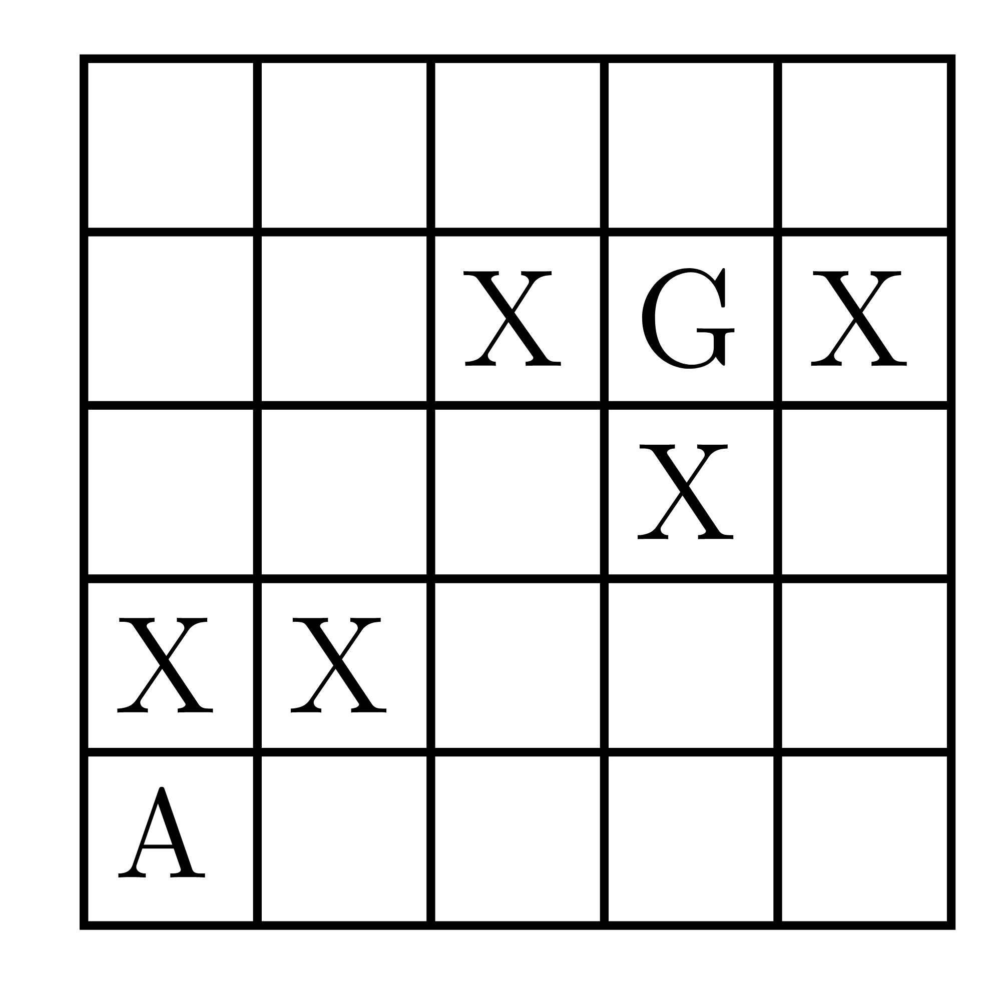Figure 7: Example to design admissible heuristic function; Agent A wants to reach to agent G.

There are 2 possible heuristic functions we can use, the Manhattan distance or the Euclidean distance. Notice that in this problem, both are equally easy to compute, but Manhattan distance provides more information because it takes into account the layout of our world while the Euclidean distance function does not. Hence, the better heuristic to use would be Manhattan distance.

3.3 Greedy-Best-First-Search

We have discussed UCS which orders the priority queue based on the estimated optimal cost $\hat{g}$ of the node from the start node, and $A^{*}$ which orders the priority queue based on the combined cost $f$ where $f(s_i) = \hat{g}(s_i) + h(s_i)$.

$~~~~~$ We can also order the priority queue based solely on heuristic function $h$ to first explore the nodes that are estimated to be closer to the goal. This approach is known as the Greedy-Best-First-Search (GBFS). It is easy to see that GBFS is not optimal and that can sometimes give bad results. Consider the graph shown in Figure 8.

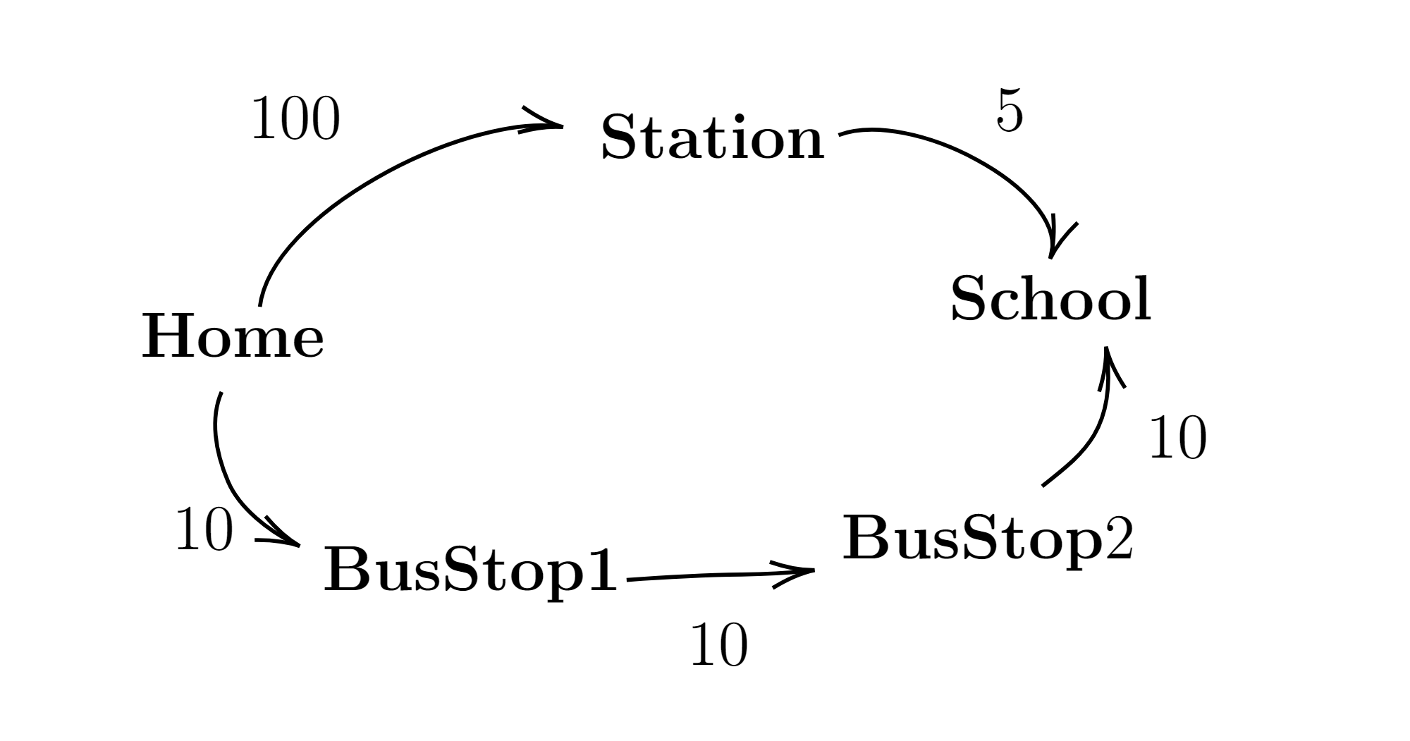Figure 8: Example to discuss Greedy-Best-First-Search; Roadmap from Home to School.

As per example Figure 8, suppose the start node is Home and goal node is School. There are two paths to reach School from Home. $Path_1$: Home, Station, School, and $Path_2$: Home, BusStop1, BusStop2, School.

Consider the following values for h:

• h (Station) = 5
• h (Bus stop 1) = 20
• h (Bus stop 2) = 10

GBFS would first explore $Path_1$, since $h(Station) = 5$ is the minimum cost in the graph. However, we see that this is not the optimal path. The cost of $Path_1$ is $105$, but the cost of Path$_2$ is $30$.