Chapter 2
2 Uninformed Search
2.1 Goal-Based Agents
In goal-based agents, the agent has a particular goal to achieve. Their environment is fully observable and deterministic. Let us reconsider the MopBot example from the previous chapter. We want the MopBot to clean such that it satisfies all performance criteria. Let us try to model the MopBot example as a goal based agent and abstract the problem using following components.
- State (of Environment): $<Location,Status(A),Status(B)>$
- Actions: ${Left, Right,Clean,Idle}$
- Transition Model: $g:State \times Action \mapsto State$
- Performance Measure: $h:State \times Action \mapsto R$
- Goal State(s): ${State_1,State_2,\ldots}$
- Start State: e.g $<Room\,A, Clean, Dirty>$
Let us assume a static environment, two locations A, B and status clean, dirty. Clean is represented as $C$ and dirty as $D$.
Figure 1 (special thanks to Khiew Zhi Kai’s class scribe) shows transition model for the MopBot example.
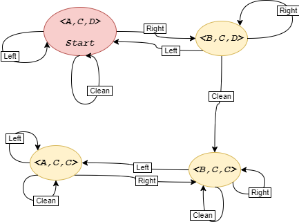
Figure 1: Transition Model for the MopBot. $A,B,C,D$ stand for location A, B, Clean and Dirty, respectively
Figure 1 represents a graph. The graph is specified implicitly because the explicit graph is very often large. In general, we specify the complexity of a graph in terms of the following.
- $b$: branching factor that is the maximum number of successors of any node.
- $d$: the minimum length of any path from start to goal.
- $m$: the maximum length of any path from start to any state in the graph.
- Performance Measure: minimum cost of the path.
The problem of goal-based agents can be abstracted as a minimum-path graph problem. Let us try to analyze an example to frame goal-based agents as a minimum path graph search problem.
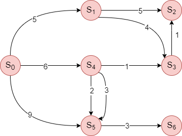
Figure 2: A graph of the transition model. A vertex represents a state, and an edge represents an action with an associated cost.
In Figure 2, we present the graph of the transition model, where each vertex represents a state and an edge represents an action with an associated cost. Let us assume that start state is $S_0$ and goal state is $S_2$. Note that goal state is not necessarily one state. The question we ask here is how to reach from state $S_0$ to $S_2$.
One possible way to find the action sequence that would reach the goal state would be to convert all possible action sequences starting from the initial state into a search tree. In the search tree, the initial state is at the root. We create a branch from any state to its subsequent child nodes by taking possible actions from that state. A search tree based on the transition model in Figure 2 is presented in Figure 3. Each node in the search tree contains information about a state, its parent, the action taken to generate the node, and its path cost.
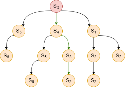
Figure 3: Search Tree corresponding to Figure 2.
To find the solution path to $S_2$, we can implement a tree-search algorithm that traverses the entire tree from the left to the right, where we terminate upon reaching $S_2$ returning the path taken from $S_0$ to reach $S_2$. The algorithm explores in the following order until it reaches $S_2$: $S_0,S_5,S_6,S_4,S_5,S_6,S_3,S_2$. Therefore, the solution path it finds would be $<S_0,S_4,S_3,S_2>$, represented by the green arrows in Figure 3.
We now focus on finding an optimal path from $S_0$ to $S_2$ in terms of time, memory, and performance measure. Our earlier search tree algorithm is not efficient. For example, the algorithm explores $S_5$ and $S_6$ twice even though visiting these two nodes cannot reach $S_2$ as there is path from $S_6$ to $S_2$. Indeed, if there is a way to remember the nodes that the algorithm has already explored, we do not need to explore $S_6$ a second time, thus improving the time and memory complexity.
Here, we ask the question: do we really need a search tree, or can we continue with the graph model shown in Figure 2?
We can traverse the graph to find a path to $S_2$, while storing the nodes already explored to avoid visiting the same node again. This can improve the time complexity, but we require more memory to remember the visited nodes. As we will see, there is a space-time tradeoff between algorithms.
2.2 Breadth-First Search
One possible way to traverse the graph would be to use Breadth-First Search (BFS). Algorithm 1 represents how BFS works.
Algorithm 1 Breadth First Search: FindPathToGoal($u$)
- $F$(Frontier)$\leftarrow$ Queue($u$)$~~~~~~~~~~~~~~~~~~$ // FIFO
- $E$(Explored)$\leftarrow{u}$
- while $F$ is not empty do
- $~~~~~$ $u \leftarrow F$.pop()
- $~~~~~$ for all children $v$ of $u$ do
- $~~~~~~~~~~$ if GoalTest($v$) then
- $~~~~~~~~~~~~~~~$ return path($v$)
- $~~~~~~~~~~$ else
- $~~~~~~~~~~~~~~~$ if $v \not \in E$ then
- $~~~~~~~~~~~~~~~~~~~~$ $E$.add($v$)
- $~~~~~~~~~~~~~~~~~~~~$ $F$.push($v$)
- return Failure
Let us try to find an optimal path to reach $S_2$ in Figure 2 through Algorithm 1. The initial state is $S_0$. The $F$ and $E$ values during each iteration would be as per Table 1 below.
| Iteration $i$ | Internal State of Data Structure |
|---|---|
| $i=0$ | $F=[S_0], E={S_0}$ |
| $i=1$ | $F=[S_1,S_4,S_5], E={S_0,S_1,S_4,S_5}$ |
| $i=2$ | GoalTest($S_2$) is true, thus return the path to $S_2$ |
Table 1: States of Data Structure $E$ and $F$.
As we now have an algorithm to find a path from the start state to the goal state, let us try to analyze the algorithm through $4$ standard criteria.
Completeness: An algorithm is called complete if and only if it is guaranteed to find a path from initial state to final state, whenever initial and final state is connected.
Claim 1: BFS is complete.
Proof:
Let us assume there exists a path $\Pi$ of length $k+1$ from the start state $S_0$ to goal state $S_g$. $\Pi : S_0, S_{i_1}, S_{i_2}, \ldots , S_{i_k}, S_g$ Note that $\Pi$ is not necessarily the shortest path from $S_0$ and $S_g$. Let us proof by induction.
- Base Case: Path of zero length, i.e $k+1 = 0$ and $S_0 = S_g$.
- Induction Hypothesis: The algorithm will find a path to all nodes where the path length $\leq k+1$.
- Induction Step: Let us assume, we are at $S_{i_k}$. Either $S_g$ is already explored or $S_g$ will be explored at time of exploring $S_{i_k}$’s children.
Optimality: The algorithm will find a path of minimum cost.
BFS is not always optimal. To understand this, let us consider the example based on Table 1, where the path solution returned by the BFS algorithm would be $<S_0,S_1,S_2>$ with a path cost of $10$. But a lower cost path would be $<S_0,S_4,S_3,S_2>$ with a path cost of $8$. Thus the returned path is not optimal.
Time Complexity: BFS will traverse all nodes in the graph in the worst case scenario. We can determine the time complexity based on the number of states in the transition model. For any general problem, the number of nodes increases by a factor of $b$ for every edge travelled away from the initial state node $S_0$. This occurs for the full depth $d$ of the graph as seen from Figure 4.
Therefore the time complexity is, $O(b+b^2+b^3+ \cdots +b^d) \leq b^{d+1} \Longrightarrow O(b^{d+1}).$
Space Complexity: In BFS, the data structure $E$ tracking which node has been explored, has to keep track of all nodes in the worst case. Therefore the space complexity for $E$ is $O(b^{d+1})$.
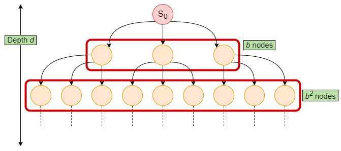
Figure 4: Number of nodes for a graph of depth $d$ and branching factor $b=3$
2.3 Breadth-First Search with Priority Queue
The BFS algorithm does not always produce the optimal action sequence as a solution. Let us modify the algorithm, where we use a priority queue rather than a queue for the data structure $F$. Algorithm 2 represents the modified BFS algorithm.
Algorithm 2 Breadth First Search: FindPathToGoal($u$)
- $F$(Frontier)$\leftarrow$ PriorityQueue($u$)$~~~~~~~~~~~~~~~~~~$ // lowest cost node out first
- $E$(Explored)$\leftarrow{u}$
- while $F$ is not empty do
- $~~~~~$ $u \leftarrow F$.pop()
- $~~~~~$ for all children $v$ of $u$ do
- $~~~~~~~~~~$ if GoalTest($v$) then
- $~~~~~~~~~~~~~~~$ return path($v$)
- $~~~~~~~~~~$ else
- $~~~~~~~~~~~~~~~$ if $v \not \in E$ then
- $~~~~~~~~~~~~~~~~~~~~$ $E$.add($v$)
- $~~~~~~~~~~~~~~~~~~~~$ $F$.push($v$)
- return Failure
The modified algorithm works such that when the node $u$ is picked from $F$, then node $u$ has the minimum cost among all unexplored nodes in the queue at that iteration.
Does the priority queue help us to find the optimal solution? We find it out for the two counter-examples raised against BFS in its optimality property above?
Counter-example 1 ($S_0$ to $S_2$): The BFS with priority queue produces a new solution of $<S_0,S_1,S_3,S_2>$ with a path cost o 10, which is still sub-optimal compared to the optimal path cost of 8 via $<S_0,S_4,S_3,S_2>$.
Counter-example 2 ($S_0$ to $S_6$): The BFS with priority queue was able to produce the improved and optimal solution of $<S_0,S_4,S_5,S_6>$ with a path cost of 11 (compared to the path cost of 12 for the BFS algorithm).
Although the modified BFS algorithm is able to get the optimal path in one counter-example, it fails to do so in another counter-example. Therefore this algorithm does not qualify for the optimality property.
This is because the algorithm returns the path to the goal state node immediately upon exploring the goal state node, which may be too early!! Moreover, by adding various nodes into the explored data structure $E$ and not exploring them again, the algorithm rules out any alternative path that may be better than the current path. In particular, there are two main issues with this approach:
- Checking for the goal state too early.
- Putting nodes in the explored set too early.
Let us try to fix the above mentioned issues. The main idea here is to keep track of the minimum path cost of reaching goal $u$ discovered so far. The algorithm is known as Uniform Cost Search (UCS).
2.4 Uniform Cost Search
Uniform Cost Search (USC) algorithm is described in Algorithm 3.
Algorithm 3 Uniform Cost Search(UCS): FindPathToGoal($u$)
- $F$(Frontier)$\leftarrow$ PriorityQueue($u$)$~~~~~~~~~~~~~~~~~~$ // lowest cost node out first
- $E$(Explored)$\leftarrow{u}$
- $\hat{g}[u] \leftarrow 0$
- while $F$ is not empty do
- $~~~~~$ $u \leftarrow F$.pop()
- $~~~~~$ if GoalTest($u$) then
- $~~~~~~~~~~$ return path($u$)
- $~~~~~$ $E$.add($u$)
- $~~~~~$ for all children $v$ of $u$ do
- $~~~~~~~~~~$ if $v \not \in E$ then
- $~~~~~~~~~~~~~~~$ if $v \in F$ then
- $~~~~~~~~~~~~~~~~~~~~$ $\hat{g}[v] = min(\hat{g}[v],\hat{g}[u]+c(u,v))$
- $~~~~~~~~~~~~~~~$ else
- $~~~~~~~~~~~~~~~~~~~~$ $F$.push$(v)$
- $~~~~~~~~~~~~~~~~~~~~$ $\hat{g}[v] =\hat{g}[u]+c(u,v)$
- return Failure
We now analyze the characteristics of UCS algorithm.
Completeness: UCS algorithm is not complete. Let us consider the case of infinite number of zero-weight edges deviating away from thegoal state. In this case, UCS algorithm will not be able to find the path to the goal state. On the contrary, if every edge cost $\geq \epsilon$ (a very small constant), the algorithm will find a path to the goal. As even if infinite such edges deviate from the goal, the summation will eventually be greater than the edge cost between start and goal.
Optimality: UCS algorithm is optimal. The main reason behind this, whenever we are performing GoalTest on a particular node, we are always sure that we have found the optimal path to that node.
Claim 2: When we pop $u$ from $F$, we have found its optimal path.
Proof: Let us use the following notations:
$g(u)$ = minimum path cost from start to $u$.
$\hat{g}(u)$ = estimated minimum path cost from start to $u$ by UCS so far.
$\hat{g}_{pop}(u)$ = estimated minimum path cost from start to $u$ when $u$ is popped from $F$.
Let the optimal path from start to goal $u$ be: $S_0, S_1, S_2,\ldots,S_k, u$. We will proof the claim using induction.
Base case: $\hat{g}_{pop}(S_0) = g(S_0) = 0$ is trivial.
Induction Hypothesis: $\forall_{i \in {0,\ldots,k}} \;\; \hat{g}_{pop}(S_i) = g(S_i)$.
Induction Step:
As we know by definition:
\(g(S_0) \leq g(S_1) \leq \ldots g(S_k) \leq g(u)~~~~~~~~~(1)\)
\(\hat{g}_{pop}(u) \geq g(u)~~~~~~~~(2)\)Therefore, by equation 1 and 2, $\hat{g}_{pop }(u) \geq g(u) \geq g(S_k)$.
Since, we have $g(u) \geq g(S_k)$, it is guaranteed that $S_k$ is popped before u.
Now, when $S_k$ is popped, $\hat{g}(u)$ is computed as follows:
\(\hat{g}(u) = min(\hat{g}(u),\hat{g}_{pop}(S_k)+C(S_k,u) )\)
\(\hat{g}(u) \leq \hat{g}_{pop}(S_k) + C(S_k,u)\)
\(= g(S_k) + C(S_k, u) ~~~~~ \text{From induction hypothesis}\)
\(= g(u)\)The estimate of u is always greater than or equal to the value of actual minimum path cost to $u$ along the path ${S_0, S_1, \cdots, S_k, u}$. \(\hat{g}(u) \geq g(u)~~~~~~(3)\)
Thus, by equation 2 and 3 \(\hat{g}(u) = g(u)~~~~~~(4)\)
Furthermore, $\hat{g}_{pop}(u) \leq \hat{g}(u)$ (note that the value of $\hat{g}(u)$ can only decrease).
Also, we know that $\hat{g}_{pop}(u) \geq g(u)$.
Therefore, we have $\hat{g}_{pop}(u) = g(u)$.
Time and Space Complexity: $O(b^{1+d}$)
UCS is guided by path cost, assume every action costs at least some small constant $\epsilon$ and the optimal cost to reach goal is C, The worst case time and space complexity is $O(b^{1+ \frac{C^*}{\epsilon}})$. 1 is added because UCS examines all the nodes at the goal’s depth to see if one has a lower cost instead of stopping as soon as generating a goal. When all steps are equal, the time and space complexity is just $O(b^{1+d})$.
We have optimality, and completeness with every edge cost $\geq \epsilon$ in UCS algorithm, but it is taking too much space. We keep all the nodes in the frontier, can we first try to go into depth? Yes, we can do depth first search, and in this case we don’t need priority queue also. We can simply use last in first out (Stack). Let us try to understand Depth First Search(DFS) in detail.
2.5 Depth First Search
The key idea in DFS is that we expand the deepest node in the current frontier of the search tree. Goaltest is conducted on the node when the node is selected for expansion. If the expanded node has no children, then it is removed from the frontier. We present Algorithm 4 for DFS.
Algorithm 4 Depth First Search(DFS): FindPathToGoal($u$)
- $F$(Frontier)$\leftarrow$ Stack($u$)
- $E$(Explored)$\leftarrow{}$
- while $F$ is not empty do
- $~~~~~$ $u \leftarrow F$.pop()
- $~~~~~$ if GoalTest($u$) then
- $~~~~~~~~~~$ return path($u$)
- $~~~~~$ $E$.add$(u)$
- $~~~~~$ if HasUnvisitedChildren($u$) then
- $~~~~~~~~~~$ for all children $v$ of $u$ do
- $~~~~~~~~~~~~~~~$ if $v \not \in E$ then
- $~~~~~~~~~~~~~~~~~~~~$ $F$.push$(v)$
- return Failure
Let us discuss the characteristics of DFS algorithm.
- Completeness: The completeness of DFS depends on the search space. If the search space is finite, then DFS is complete. However, if there are infinitely many alternatives, we might not find a solution.
- Optimality: DFS is not optimal.
- Time Complexity: For graph search, the time complexity for DFS is bounded by state space $O(V)$ where $V$ is a set of vertex and $V$ may be infinite. However, for tree search, we may generate finite $O(b^m)$ nodes in the search tree, where $m$ is the maximum depth of any node and $b$ is the branching factor (still, $m$ might be infinite itself!!).
- Space Complexity: $O(bm)$ where $b$ is the branching factor and $m$ is the maximum depth.
Hence, it turns out that there is a trade-off in DFS algorithm. We are losing in terms of completeness, and optimality, while we have a significant improvement in terms of space.
So far, we have discussed BFS, UCS and DFS algorithms. There is one thing common in all three algorithms; in all algorithms, we do not have any information about the goal. This type of search, where we do not have any information about the goal is known as uninformed search. The obvious question we may have now is: does the information about goal help?. Let us discuss one informed search algorithm called $A^{*}$ algorithm in the next chapter.